Quaternions and Volume Registration -- A Comprehensive Approach
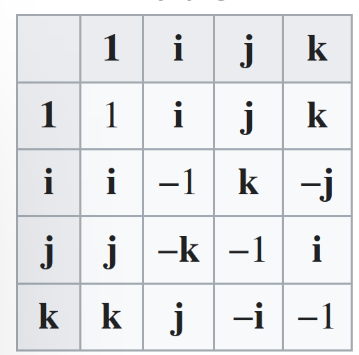
 Suppose you have two point-sets in 3-D space, related by a rotation and translation – in the presence of some noise, how can you determine this relationship given only the point-sets? This problem is one of registration, i.e. determining which points in each point-set correspond to one another. Quaternions are very useful for representing 3-D rotation, but their use in solving this registration problem is poorly, and sometimes erroneously documented. In this post, I wish to provide a more comprehensive view of how quaternions function, and their role in volume registration, as well as correct one publication's major errors. Image: The product relationships for the quaternion basis elements, 1, i, j and k.
First I will describe the motivation for solving the 3D registration problem. Then, I will derive an algorithm for computing the optimal registration. Along the way, I will provide a comprehensive review of the algebra of quaternions, with special attention paid to versors used to define 3D rotations. I will then show some promising results on synthetic and in vivo volumes. Lastly, I will describe the many errors of the presentation of the algorithm derivation in Dolezal et al, 2020. Throughout this post, I will make use of Julia's Symbolics.jl computer algebra package.
Motivation
Consider the following scenario – you and your friend see your cat doing something adorable, and take picture of it at the same time. Now, looking at the pictures, could you tell me where the two cameras were positioned? In three dimensions, instead of images, these would be volumes, or 3D point-sets.
As I've discussed before on this blog, my research focuses on using OCT to reconstruct displacement measurements. This is done via measuring a single structure at multiple known angles. In practice, this is done by measuring vibrations within a large 3-D volume of positions, rotating the preparation, and then repeating the measurements at this new angle. To reconstruct the motions, we then must ask – how are these two volumes related? Which positions correspond to one-another between volumes?
Formulation in the special case of known correspondence
In OCT, as in many modalities, the angle greatly impacts the "lighting" of the image. That is, structures which are extremely bright at one orientation may appear dimmer at other orientations, as the object may be further from the focal point of the lens or obscured by other structures along the way. As a result, we choose to work with binary volumes, which are thresholded so that sufficiently bright pixels are represented by 1s and dimmer pixels are represented by 0s. For the remainder of this section, we follow the development of Horn et al closely.
Let's call the first volume point-set , which we will represent as an matrix whose columns represent the coordinates at which there is sufficiently bright signal (a 1) in the first volume. Similarly, let be the second such set, size . In practice, and will almost always be different, and we do not know how the points relate to one another. However, we can formulate the special case of the problem where we do know this relationship, and .
In this case, we know that each point in , , is a rotated and translated version of the corresponding point in , . That is, we can write
The unknowns here are and . is a rotation in three-dimensional space, which we are careful to write as a function rather than a matrix. This is a unitary linear operator, which has a matrix representation, but as we will show soon can also be represented by quaternions. The vector represents a translation.
In the presence of noise, this becomes an optimization problem, where we look to find and that minimize the mean square error:
Solution for the translation vector
We are maximizing this real expression in two variables, and . It is preferable to split this into two optimization problems, each in one variable. To do so, we first shift both and so that they are centered at their respective centers of mass. The centers of mass are
and the new shifted coordinates are
Writing the error terms using these coordinates gives
where is independent of . We have used the fact that is a linear operator. Now we can expand the squared error terms in the standard manner:
where we have made use of the fact that is -independent in the second and third term. First, we will tackle the third term:
where we have employed the definitions of the centers of mass and primed coordinates, as well as . This means our error formula now has only two terms:
The first term is entirely independent of (and ). The second term is minimized when , or
Conceptually, this formula is intuitive – the optimal translation is the one that makes the centers of mass coincide! Note that while this formula depends on , this form of will minimize the last term of no matter what is. Moreover, it does not result in a further restriction on . That is, the terms can safely be handled as two separate optimization problems (one of which we have now solved).
Handling the rotation operator
To determine the optimal , we look to the first term in our expression for . That is, we want to minimize
Now if we were to treat as a unitary matrix, we would continue to procede down the path seen developed in Horn et al. The result is that if you define
the cross-covariance matrix of and , then the optimal rotation is
This can also be computed using the spectral value decomposition for (see the Kabsch algorithm).
While this solution is sufficient, computing a matrix inverse square root or a spectral value decomposition is not ideal. Moreover, matrices are only the second-most elegant way to describe 3-D rotations. Let's put a pin in Equation 10 for now, and we'll derive a second way to minimize it.
Representing rotations using numbers– 2-D foundations
To tackle the problem above – minimizing – with quaternions, we first need to learn what a quaternion even is. Let's start with the complex numbers, where and . This may seem elementary, but I believe this derivation is necessary to motivate the quaternions. Feel free to skip this if you feel comfortable already. Under this definition, the complex numbers form a field, i.e. a set of numbers with
a) Associative and commutative addition and multiplication operations
b) Distributivity of multiplication over addition ()
c) A unique additive identity element ()
d) A unique multiplicative identity element ()
e) Unique additive and multiplicative inverses for every element (1/x and -x, save 0, which has no multiplicative inverse).
It is easy to see that forms a field. We can represent a complex number as an ordered pair of two real numbers , suggesting a representation as a two-vector in Cartesian space. This is called the rectangular form. In this form, addition corresponds to vector addition. What does multiplication correspond to?
To see this, we need a third way to think about complex numbers – polar form. We can write any two-vector in Cartesian space both as , its rectangular components, or as , its magnitude and phase in the standard 2-D sense, , .
The product of two complex numbers and in rectangular form is . It can be quickly shown that in polar coordinates, this is precisely . That is, multiplying two complex numbers 1) multiplies their magnitudes and 2) adds their phases. See the CAS code below, where is the product performed in this way, and is the product performed via standard complex product. They are equal by simple expansion:
function cprod(z,w) 	     	     # Complex product
	[(z[1]*w[1]-z[2]*w[2]) (z[1]*w[2]+z[2]*w[1])]
end
function polar(z) 	     	     	 # polar form from rectangular form
	[sqrt(z[1]^2 + z[2]^2) atan(z[2],z[1])]
end

@variables  z_r z_i w_r w_i
zwpolar = latexify(polar(cprod([z_r z_i],[w_r w_i])))
pz = polar([z_r z_i])
pw = polar([w_r w_i])
zwcheck = latexify([pz[1]*pw[1] pz[2]+pw[2]])Now let's consider a new set, – the set of unit-magnitude complex numbers. This is the complex unit circle group – it is not a field, because if you add two numbers in the set you get a number outside the set. Multiplication of any complex number by a vector corresponds to a rotation by the argument of . Consider also a mapping defined by
This mapping is injective and surjective, so it has an inverse which maps back the complex pairs to their corresponding real vectors. The mapping is also magnitude- and phase-preserving, as magnitude and phase are identically defined for real vectors and complex numbers in rectangular form.
It is often desirable to rotate a 2-D vector, and this process is usually described by left-multiplication of the column vector by a unitary 2-D matrix, , the special orthogonal group. However, this matrix has four elements, which is a bit clunky and inelegant. We can see now that this rotation can just as well be described via multiplication by a unit complex vector. Let be real vector rotated counter-clockwise by . Let be the unique unit complex number with argument . Then
This elegant formulation allows each 2-D rotation to be uniquely described by a single unit complex number, as opposed to a matrix – a two-parameter rotation, rather than a four-parameter rotation.
Enter Quaternions
Complex numbers are nice in 2-D registration problems as they allow us to rotate coordinate vectors in a compact and elegant manner, but unfortunately they do not work in our 3-D world. Our goal is instead to derive a set of numbers where multiplication corresponds to 3-D rotation under an invertible mapping, ideally more compact than the unitary matrices in .
In my college complex analysis and modern algebra courses, I was introduced to the idea of quaternions, a four-dimensional extension of the complex numbers which is used to describe rotations in . In extending to higher dimensions, computations become complicated and you lose multiplicative commutativity. I tossed aside the concept as a pure-mathematics pipe dream, but now, five years later, I am reaping what I've sown.
The quaternions, (for Hamilton, their noble father), are defined as the four-dimensional set of numbers , where and , and are called the basic quaternions. The basic quaternions satisfy the following relationship:
That is, each of the basic quaternions is, in a sense, an imaginary unit. How they differ from one another lies in the third term – recalling that quaternions are not commutative under multiplication, this set of equalities actually gives 16 identities for the products of quaternions. For example, while . It is very impotant to note that the quaternions are not anticommutative – there is no quick way to determine from for two quaternions. You could think of this as analogous to matrix multiplications, which are similar in this regard.
We can add two quaternions componentwise, meaning quaternion addition is commutative and associative, has an identity element (0) and has additive inverses for every element (by negating every component). This means that is an abelian group (or commutative group) under component-wise addition.
We can multiply two quaternions by distributing the components, taking into account order of the basic quaternion products. This is called the Hamilton product. Note that the real coefficients are still commutative with the quaternions. Representing the real, , and components as components in a vector, we can write:
function hamprod(q,w) 	     	     # Hamilton product
	[q[1]*w[1]-q[2]*w[2]-q[3]*w[3]-q[4]*w[4]
	 q[1]*w[2]+q[2]*w[1]+q[3]*w[4]-q[4]*w[3]
	 q[1]*w[3]-q[2]*w[4]+q[3]*w[1]+q[4]*w[2]
	 q[1]*w[4]+q[2]*w[3]-q[3]*w[2]+q[4]*w[1]]
end

@variables  q_0 q_1 q_2 q_3 w_0 w_1 w_2 w_3 i j k
qw = hamprod([q_0 q_1 q_2 q_3],[w_0 w_1 w_2 w_3])
qw = latexify(qw[1]*1 + qw[2]*i + qw[3]*j + qw[4]*k)Where is just . It can be seen from the expression above that this product is associative and distributes over addition, but is not commutative. This means is not a field. However, we will show that you can divide quaternions, so that all non-zero quaternions have unique multiplicative inverses. This makes a division ring, which is similar to a field (described above) barring only the commutativity of multiplication.
We will now develop quaternion division. It is conventional to write quaternions as column vectors consisting of their four real coefficients,
For such a , we define its conjugate, as follows:
This is analogous to the complex conjugate. We define the norm or modulus of a quaternion in the same was as that of a four-vector:
Showing the second equality is not too difficult from the definition of quaternion product. One clear upshot of this is that the modulus of a scalar (real) quaternion is . The modulus is multiplicative, which means that if and are two quaternions, then
Showing this is not challenging with a computer algebra system, but is a pain by hand. We show this for the square modulus which is simpler to visualize:
function QuatModSq(q) # quaternion modulus squared
	q[1]^2+q[2]^2+q[3]^2+q[4]^2
end

@variables  q_0 q_1 q_2 q_3 w_0 w_1 w_2 w_3
qwmodsq = QuatModSq(hamprod([q_0 q_1 q_2 q_3],[w_0 w_1 w_2 w_3]))
qmodwmodsq = QuatModSq([q_0 q_1 q_2 q_3])*QuatModSq([w_0 w_1 w_2 w_3])
equalitycheck = isequal(qmodwmod,qwmod)
@show(equalitycheck)
Failed to precompile Symbolics [0c5d862f-8b57-4792-8d23-62f2024744c7] to /home/runner/.julia/compiled/v1.7/Symbolics/jl_JHGFna.
Of course, as the moduli are real numbers, this commutes. Now we define the unit sphere group in quaternion space, more commonly called the versors. I will denote them as , defined as
The versors form a group under multiplication, by the multiplicativity of the modulus. It can be shown that the product between a versor and its conjugate is – the multiplicative identity! That is, if is a versor, then
This allows us to define versor division, i.e. for versor , its inverse is . We will now use this to define quaternion division. We can write any non-zero quaternion as the product of its norm and a versor,
The versor on the right has an inverse which is its own conjugate, and scalar multiplication can be absorbed into the conjugate, so we can write
This defines the quaternion multiplicative inverse and thereby quaternion division:
Finally, quaternions can be mapped to matrices in an incredible way! Let be defined by
We use capital letters to denote corresponding matrices for our quaternions. This formalism is incredibly important for our development, so be sure you follow along. This mapping is an isomorphism, which means that is invertible and for any quaternions and , we have .
Another incredible feature of this representation is that it allows us to treat quaternions as real column vectors. Consider the boring mapping defined as
It is clear that the inverse of will look exactly the same, but will map from real vectors to quaternions. One can think of it as "reading the quaternion as a vector." Then I can write for any two quaternions
That is, I map the first quaternion to a real matrix and the second to a vector. Their product is a vector, which I can read as a quaternion through the inverse mapping of (which looks like an identity mapping). An abuse of notation would be to write this as:
where we are reading as a real vector and the output of the right-hand side as a quaternion. That is, the and mappings are to be inferred.
Below, we show that the Hamming product, the product through multiplying quaternion matrices, and the product of a quaternion matrix and a quaternion column vector are the same:
function QuatMat(w) 	     	     # Create matrix form of a quaternion
	[w[1] -w[2] -w[3] -w[4]
	 w[2]  w[1] -w[4]  w[3]
	 w[3]  w[4]  w[1] -w[2]
	 w[4] -w[3]  w[2]  w[1]]
end
function Mat2Quat(A) 	     	     # Grab quaternion from matrix form
	[A[1,1] A[2,1] A[3,1] A[4,1]]
end

@variables  q_0 q_1 q_2 q_3 w_0 w_1 w_2 w_3

MatProdMethod = Mat2Quat(QuatMat([q_0 q_1 q_2 q_3])*QuatMat([w_0 w_1 w_2 w_3]))
HamProdMethod = hamprod([q_0 q_1 q_2 q_3],[w_0 w_1 w_2 w_3])
ColProdMethod = QuatMat([q_0 q_1 q_2 q_3])*[w_0;w_1;w_2;w_3]We also have (this is clear from the definition. This allows us to turn the quaternion multiplication into real matrix multiplication, which allows us to use known theorems from linear algebra.
Quaternion representations of 3-D rotations
Finally, we will use quaternions to represent 3-D rotations, analagously to how we used complex numbers to describe 2-D rotations. First, lets define a mapping by
Let be the axis (as a unit vector) about which we would like to rotate vector , and let be the angle by which we would like to rotate . The matrix in that decribes this rotation is
This alone should make it clear that the rotation matrix is an ugly animal to work with. Instead, we would like to work with quaternions. A rotation is a unitary linear operation, so it cannot change the norm of the input. As such, we will specifically work with versors (quaternions with unit magnitude).
We can write the vector which is conjugated by versor as
One can show that for , this expression can equivalently be written as
Check out the expressions below – they are equal if you insist is unit norm:
@variables  a b c d v_x v_y v_z

QMatMethod = Mat2Quat(QuatMat([a b c d])*QuatMat([0 v_x v_y v_z])*QuatMat([a -b -c -d]))
QMatMethodW = QMatMethod[2:4]
RMat = [1-2(c^2+d^2) 2*(b*c-d*a)   2*(b*d+c*a)
		2*(b*c+d*a)  1-2*(b^2+d^2) 2*(c*d-b*a)
		2*(b*d-c*a)  2*(c*d+b*a)   1-2*(b^2+c^2)]
RMatMethodW = RMat*[v_x;v_y;v_z]Letting
we have that the matrix generated via conjugation by is precisely the rotation matrix about axis by angle presented above. This can be seen by plugging in the coefficients and making use of trigonometric identities, as well as the fact that is a unit vector.
This gives us a four-parameter versor method for computing rotations, as opposed to the nine-parameter behemoth of using the representation. I believe this is the more compact and elegant way to tackle the problem at hand.
Solving for the optimal rotation operator – the quaternion way
Did you forget what we were doing? We were looking for a quaternion method to solve Equation 10 above, as opposed to the referenced method. This method is poorly documented, and I believe it is high time to change that fact.
The solution is presented rather elegantly in Besl and McKay, but it is not derived. The authors cite Horn et al, who we followed to derive both the optimal translation vector and Equation 10. However, they follow from this point to derive the optimal rotation matrix in . This is precisely what we are trying to avoid.
The authors also cite Faugeras and Hebert, who do present a quaternion method, but arrive at a different form of the solution than Besl and McKay (they formulate an eigenvalue minimization problem, while Besl and McKay formulate an eigenvalue maximization problem).
Benjemaa and Schmitt do provide a derivation of a solution analogous to that of Besl and McKay, but with a slightly different framing of the problem. Moreover, the notation is a bit inelegant and the approach is hard to follow.
Finally, Dolezal et al in their 2020 EANN conference paper attempt to arrive at the same result, but make an upsetting amount of theoretical errors. I will cover this in more detail shortly.
I will follow the first step of Faugeras' approach, and then abandon all literature and do everything on my own. Let's begin with Equation 10 again, but we will write the rotation operator in terms of a quaternion :
where and – that is, they are the quaternion representations of these vectors. As the expression inside the modulus has real component 0, the quaternion modulus is identical to the two-norm of the corresponding vectors. This means , as desired. We are looking for versor that minimizes this expression.
To begin, we use the fact that the quaternion modulus is multiplicative, and multiply by the squared modulus of . As is a versor, this is equivalent to multiplying by 1. Using the fact that for versors, , this allows us to write:
From here, we expand out the squared norm. This turns out to be identical to expanding the square norm of a vector difference, where the quaternion dot product is identical to the dot product on (this is not hard to show by writing out terms, if you are interested). Note that this means the dot product is commutative. We have
We have used the multiplicativitiy of the quaternion modulus and the fact that is a versor. The first two terms are -independent, so minimizing is equivalent to minimizing the third term. The term is negative, so this is equivalent to maximizing the negative of this term. That is,
Maximizing the term on the right is our new goal. First, we will use our matrix representation of quaternions to map this quaternion expression to one containing only real matrices and vectors:
To proceed, we need one more identity. This looks close to the form of a quadratic form , which invites optimization via eigendecomposition. However, to arrive at this form, we would need to swap the order of and , which is illegal! We instead must use the restrictions in place to arrive at a new matrix, , such that .
We will work this out "by hand" here, despite its seeming silliness, because this is not present in any literature I have found. If and , we can write
This is not merely the transpose of . Now we can write the expression to be maximized as
Pulling the -independent vector-form versors and out of the sum turns this into a quadratic form. It can be shown computationally that is a symmetric matrix (I used a computer algebra systemi just to make sure).
The problem comes down to maximizing a quadratic form defined by a symmetric matrix, constrained by . The solution to this sort of problem is well-known, and is derived through the spectral theorem. The spectral theorem states that any symmetric matrix is unitarily diagonalizable by a matrix whose columns are the unit eigenvectors of . Moreover, the entries on the diagonal of the diagonal matrix are the eigenvalues of . is orthonormal, so . Letting , we can write the quadratic form above as
where the are the eigenvalues of and the elements of are, by definition of , the projections of onto the eigenvectors of . We write where is the unit eigenvector of corresponding to eigenvalue . Without loss of generality, assume is the largest eigenvalue of . Because is of unit norm, it can be seen that the expression above will reach its maximum value when . This occurs if , or . That is, the optimal rotation quaternion is the unit eigenvector of corresponding to the largest eigenvector.
Now we have found the optimal rotation in terms of quaternions, incredibly, via solving a real eigenvalue problem! This is the wonder of representing quaternions as real matrices. In contrast, using matrices, we would have to compute a spectral value decomposition. Generally speaking, eigendecomposition is significantly faster than SVD.
An attractive closed form for
We can write this matrix, as Besl and McKay do, in terms of the cross-covariance matrix very neatly. I will mimic their notation. The cross-covariance matrix is
Its antisymmetric component (times 2) is . Let . Then we can write our matrix of import as
where is the identity matrix. Note that in both the and quaternion methods, we must compute the cross-correlation matrix. This formula for makes it clear that no other significant computation is required to arrive at . The concurrence between this expression and the one derived above can be shown, but is best done via a computer algebra system. We do so below, showing the summands in Equation 51 rather than the entire matrix. This is equivalent to showing equality of the sums. SBesl is a summand in Equation 51, and SFrost is a summand in Equation 48:
@variables  x_1 x_2 x_3 v_1 v_2 v_3 SIGMA A DELTA SBesl SFrost

x = [x_1;x_2;x_3]
v = [v_1;v_2;v_3]
XMat = QuatMat([0;x])
VMatHat = [0   -v_1 -v_2 -v_3
		   v_1  0    v_3 -v_2
		   v_2 -v_3  0    v_1
		   v_3  v_2 -v_1  0]
SIGMA = v*transpose(x)
A = SIGMA - transpose(SIGMA)
DELTA = [A[2,3];A[3,1];A[1,2]]
SBesl = [tr(SIGMA) transpose(DELTA)
     DELTA SIGMA+transpose(SIGMA)-tr(SIGMA)*[1 0 0;0 1 0;0 0 1]]
SFrost = transpose(XMat)*VMatHat
@show latexify(SBesl)
@show latexify(SFrost)
@show isequal(SBesl,SFrost)The case of unknown correspondence
All of this was to determine the optimal translation and rotation when the correspondence of the points between the sets is already known – that is, the points are already registered. Part of our problem is actually registering the points! Don't worry, this won't take too long...
We present Besl and McKay's algorithm. Suppose we start with sets and each with a different number of points. For each of the points in , we will find the nearest point to it in , consider those two points registered. This allows us to define a new registered point set of ordered points in :
We call the ordered set of such points the set of closest points in to , and write it as a matrix. Now we are in the special case where we have two equally sized registered sets of points, so we can use the algorithms described above!
Of course, this is very naive at first glance – assuming that the nearest points are registered is clearly invalid in even the most basic of examples. However, in an iterative algorithm, we can perform the registration again after our first rotation and translation to gain a better sense of the true registration.
At each iteration, we will change the target/registered set based on the formula above, then carry out our algorithm as described above. This is:
Initialize , , , and =0. The following steps are then repeated, iterating over until convergence is achieved.
1 – Compute the closest points in to , , as well as the mean squared error . Terminate the algorithm if is sufficiently small.
2 – Compute the optimal rotation and translation for these vectors via either the quaternion or methods described above.
3 – Apply the rotation and translation: .
This algorithm will converge to a local mean squared error minimum. While this is proven by Besl and McKay, this should already be convincing – at each the error between and is minimized via the closest points operation , and then the error between and is minimized by finding the optimal rotation and translation (as proven above). It should be clear that this "chain of minimization" will never increase the error.
Results for OCT volumes – Synthetic ellipsoids
I have seen promising results using this algorithm, both using synthesized "perfect" data and real data from the round window membrane from an in vivo gerbil experiment. I will present the perfect data first. Unless otherwise stated, all volumes are displayed with MATLAB's volume viewer, and all computations are done with MATLAB. I made heavy use of the MATLAB image processing toolbox.
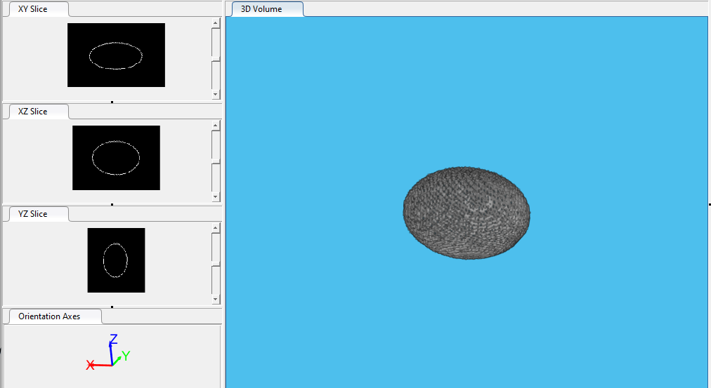
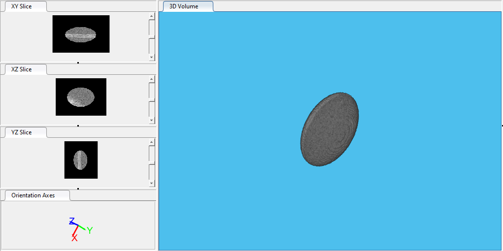 I began with a volume scan of a speaker membrane, which is thick, reflective and flat. I then thresholded this data by index to form an ellipsoidal solid, as shown to the left. We will rotate, translate and add noise to this volume. This will generate a second volume, which we will try to register with the first.
Below we plot the two volumes, initial and transformed, on top of one another. These are not binary volumes, but rather unsigned integers. We have to turn these into binary volumes so we can form two lists of indices, and . We also should note that the algorithm has super-linear complexity in , so we want to reduce the number of points in and as much as possible without losing the information necessary to register the volumes.

Our solution is to a) downsample the volume so that there are fewer total points; b) median filter the volume to denoise – we are not concerned with fine features, so this is ok; c) threshold the image to make it a binary one containing only the most reflective structures; d) segment the volume, as registering one segment in the volumes should be equivalent to registering the volumes in total; e) perform edge detection, as registering the segment's edges is equivalent to registering the segment, which is equivalent to registering the entire volumes.
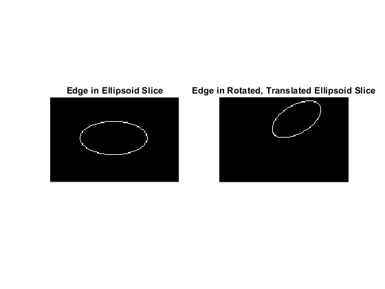
It is much easier to look at cross-sections, as humans have a hard time visualizing three-dimensional objects from images alone (weak). Here is a single cross-section of the two volumes after the process above has been employed. The effects of translation and rotation are visible through these two images. We call these two sets of 3-D edge points (unrotated) and (rotated/translated). In this case, contains 10150 points and contains 9971 points, whereas the thresholded images have about 100000 points.
 Let's consider the first step in the algorithm, where we start by computing the first pairing between and a subset of called . The set is shown to the left, which we can see is all on one side of the ellipsoid. This is because the rotated ellipsoid is on one side of , so all of the points on are nearer to these points than ones on the opposite side. This should "fill out" as we proceed across more iterations.
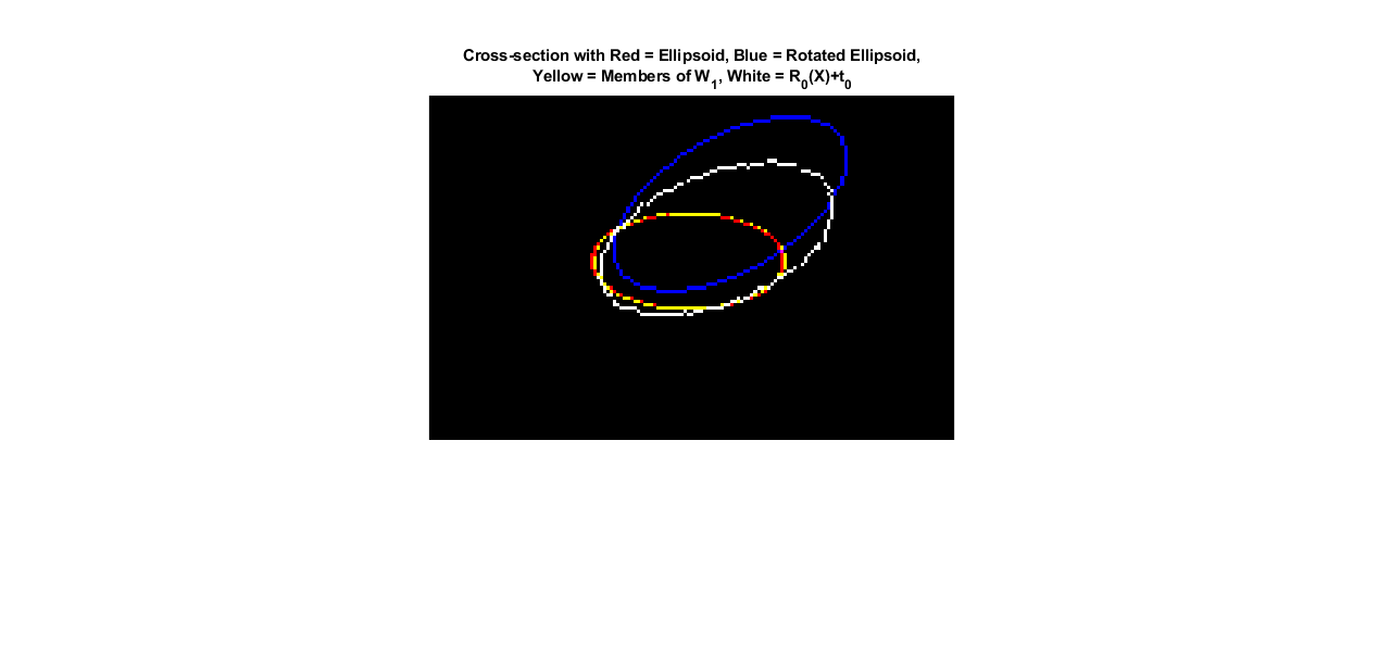 The next step is that we compute the first optimal rotation and translation to register with , yielding . The image to the right presents an example cross-section containing in red, in blue, in white and the new nearest set in yellow. You can see that the white ellipsoid, the first registration attempt, is nearer to the correct shape of than the original . The new nearest set, , is no longer on only one side of the ellipsoid. Note that this rotation does not preserve cross-sections, so do not be misled!.
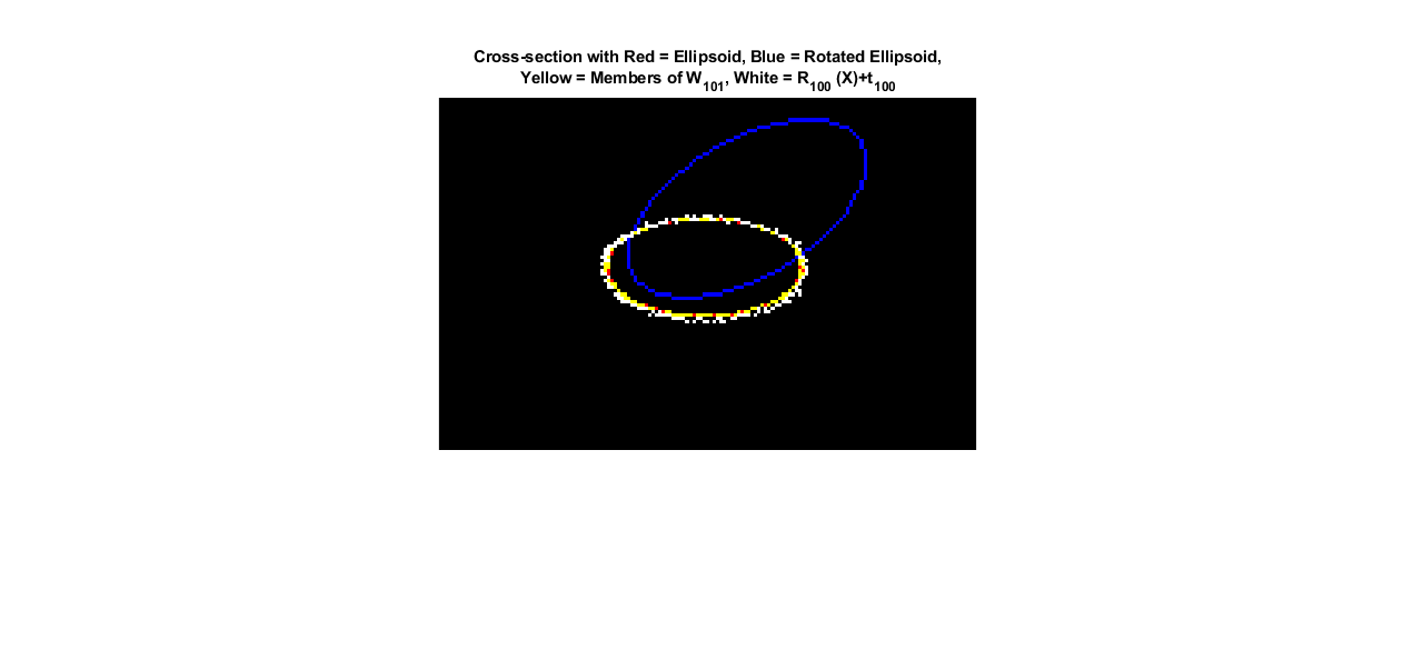
Finally, we will Consider what happens after 100 iterations. The figure below is of the same type as that above. The white cross-section – the approximate registration after 100 iterations – is nearly right on top of the target volume ! This is exactly what we want. To be sure this holds across all cross-sections, we plot the two volumes on top of each other below. They are directly on top of each other, near-indistinguishable. On my not-so-great computer, 100 iterations took 85 seconds.
Finally, let's look at the convergence of the mean square error. The figure below shows that in this idealized example, the error approaches zero quite rapidly. The figure below this one, however, tells an interesting story. Although the error remains very low, changing by tiny fractions of a percentage point after 25 iterations, the translation and quaternion vectors actually change very significantly after this point – and , for example, change by 50\% between 25 and 100 iterations. This is because the geometry of the problem.
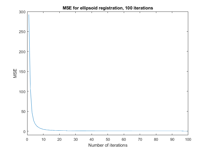
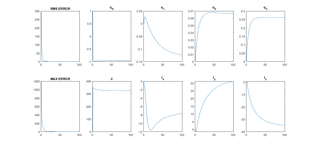
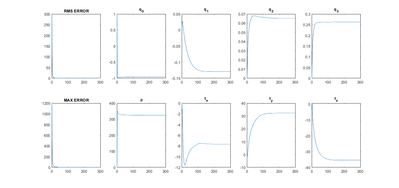
This means that converged error is not actually the best metric for converged registration. Instead, we should determine converges by percent change in every element of and . This effect exaggerated because of the geometry of this problem, but is necessary to watch out for. Below, we show the convergence curves after 300 iterations, after which all parameters have converged.
Results for OCT volumes – an in vivo gerbil cochlea
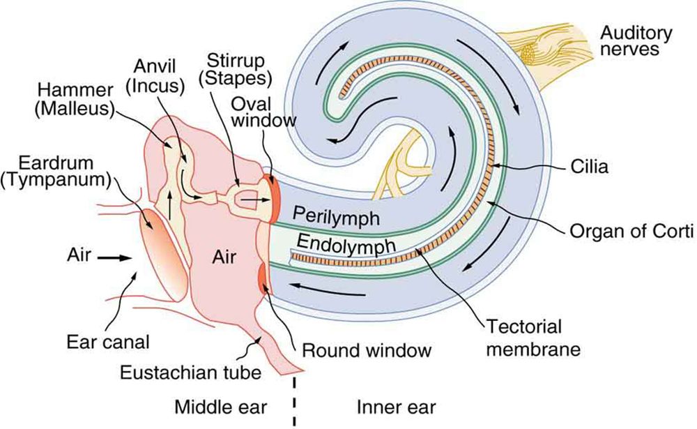 In our lab's in vivo gerbil experiments, we take vibration measurements through the round window membrane (RWM). The RWM is a transparent structure atttached to the bony wall of the cochlea, through which the organ of Corti can be seen (see the anatomical diagram to the right). The OCT beam cannot penetrate the bony wall, as it is not sufficiently transparent. This means that portions of the organ of Corti may be visible at some angles but not others.
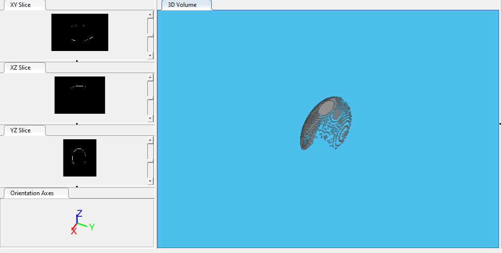
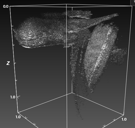
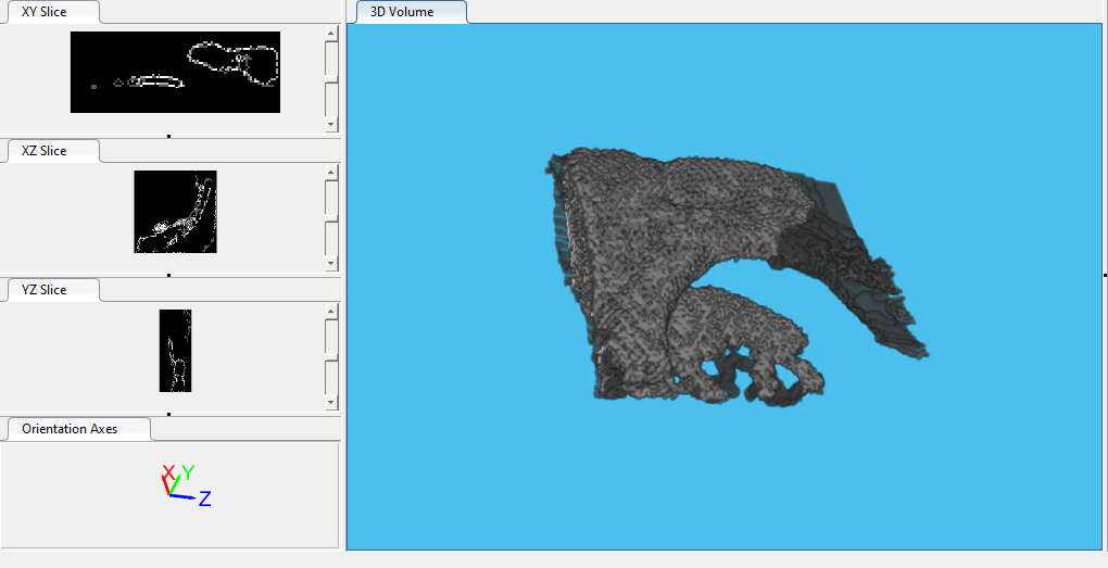
However, the RWM and bony wall's surface always get light. This means that when we are trying to register two cochlear volumes, while we are only interested in vibrations within the organ of Corti, we will register using the RWM and bony wall. Consider the volume scan below, presented in the ThorImage software. It is a bit challenging to parse, but the band spiraling downward (in ) is the organ of Corti. The top part is RWM and bone.
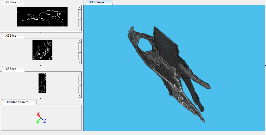 That means that in our pre-processing, we need to segment out the RWM and bony wall. I have rotated and translated one RWM volume, added noise and then carried out this pre-processing. The segmented RWM and bone volumes are presented atop one another in the image to the left.
This is very hard to parse because the shapes are far more abstract. However, the cross-sectional images are much easier to visualize. Below are the registered cross-sections after 300 iterations, the error over iterations and the registered volumes on top of one another.
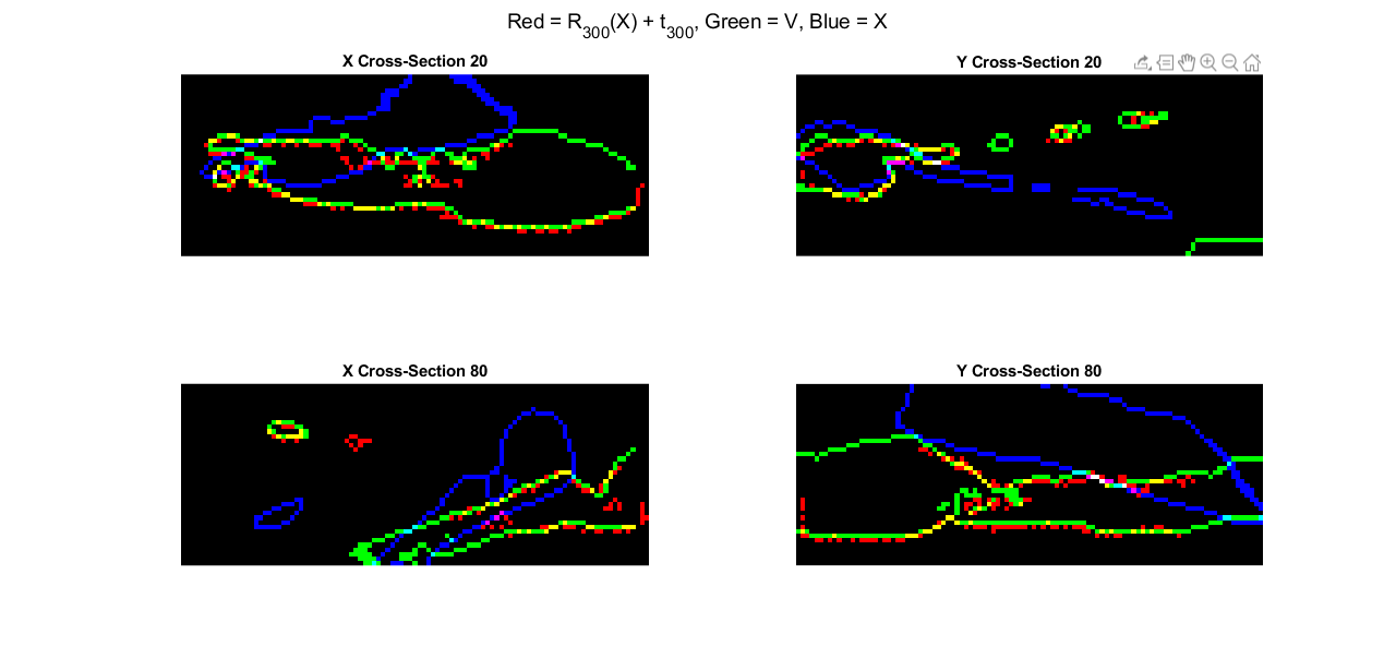
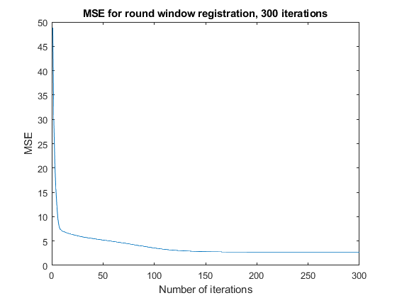
Note that convergence is slower, and due to the more abstract shapes, noise affects the minimum error more. This is beautiful and promising operation for in vivo cochlear volumes!
My gripes with Dolezal et al
I am very dissapointed in a conference paper published by Dolezal et al in the Proceedings of the EANN 2020 Conference, which includes massive falsehoods in computing the optimal quaternion rotation matrix. I will walk through all of them here.
1 – Inventing a quaternion dot product identity
Start with their Equation 10, which is an expanded version of the error equation we provided above. They correctly say they should maximize the second term, then write the following in Equation 11:
where , and are quaternions. This statement implies that quaternions distribute in an interesting manner across dot product, even when and have only vector parts.
This is verifiably false, as I will show with the CAS below:
@variables  a_x a_y a_z b_x b_y b_z q_0 q_1 q_2 q_3 LHS RHS

q = [q_0 q_1 q_2 q_3]
qconj = [q_0 -q_1 -q_2 -q_3]
a = [0 a_x a_y a_z]
b = [0 b_x b_y b_z]

LHS = dot(hamprod(hamprod(q,a),qconj),b)
RHS = dot(hamprod(q,a),hamprod(b,q))
equalitycheck = isequal(LHS,RHS)2 – Falsely claiming a matrix is symmetric to apply the spectral theorem
The authors then give the correct forms for quaternion matrix representations (as seen in my presentation above) in equations 12 and 13. If their Equation 11 were correct, their expression of the dot product as a quadratic form in would be valid (their Equation 14).
However, they claim that the matrix is symmetric, where and represent the matrix form of the quaternions and . Taking this product gives a matrix which is clearly not symmetric! In fact, its off-diagonal elements are skew-symmetric! See below:
@variables  a_x a_y a_z b_x b_y b_z
AtB = latexify(transpose(QuatMat([0 a_x a_y a_z]))*QuatMat([0 b_x b_y b_z]))We thereby cannot employ the spectral theorem and cannot say the maximum eigenvalue's unit eigenvector is the optimum quaternion, as they do in their Equation 15.
3 – Falsifying a matrix product, and a probable typo
How do they get around this? They simply falsify an expression for not equal to . That is, their equation 16 is simply not We computed this above.
They also claim that the matrix they present is symmetric, but it can clearly be seen that the and entries are not equal! Sure, this could just be a typo. In fact, correcting for the minus sign in the entry, their matrix is precisely that presented in my Equation 43, and in Besl and McKay!
It is more than likely that the authors simply (mis)copied the final matrix from a publication similar to Besl and McKay, and then fabricated a mathematical reasoning to pretend to arrive at the correct result. The rest of their publication seems to carry around this sign error.
Their result – that the computational complexities of the and quaternion-based algorithms are the same – is consistent with what I've seen empirically. The two methods seem to take similar amounts of time to run in my environment. My gripe is not with their result, but their presentation.
My anger comes from the fact that a derivation of the optimum quaternion like the one I have presented above is very difficult to find. Having to gain familiarity with quaternion arithmetic to attack this problem, I was stalled and confused by this article.
Ultimately, in deriving the result on my own, I recognized that almost all of their steps contained major errors, and I think that this should not have been published in its current form. It is not correct and it is not fair to the reader, especially in this context where the material is very difficult to find elsewhere.
I know it is not likely, but I would like to call on Springer Nature to publish at least an errata for this publication. Hopefully my accurate and comprehensive presentation, while lengthy, could help people in my position who are looking for a derivation of this type.
© brian l frost. Last modified: October 02, 2023. Website built with Franklin.jl and the Julia programming language.